ANTsR TUT
Leonardo Cerliani
18 February, 2021
Before you start
This tutorial for ANTsR is based on the Rmd notebook by Brian Avants on antsRegistration in R.
The Rmd version was evaluated riding on the Storm, but it should work everywhere.
Read images
library(ANTsR)
library(ggplot2)

# Read images
r16 = antsImageRead( getANTsRData( "r16" ) )
r64 = antsImageRead( getANTsRData( "r64" ) )
Visualization
Define functions for plotting
# Only one image
antsplot.single <- function(image){
  invisible(
    plot(
      image,
      doCropping = F
    )
  )
}


# Simple overlay with alpha
antsplot.olay <- function(bg, olay, alpha=0.5){
  invisible(
    plot(
      bg, olay,
      color.overlay='red',
      doCropping = F,
      alpha=alpha,
      window.overlay = quantile(olay, c(0.72,1))
    )
  )
}


# Overlay canny borders
antsplot.canny <- function(bg, olay, alpha=1){
  canned_olay = iMath(olay, "Canny", 3,3,3)
  invisible(
    plot(
      bg, canned_olay,
      color.overlay='red',
      doCropping = F,
      alpha=alpha
    )
  )
}
Plot single image
antsplot.single(r16)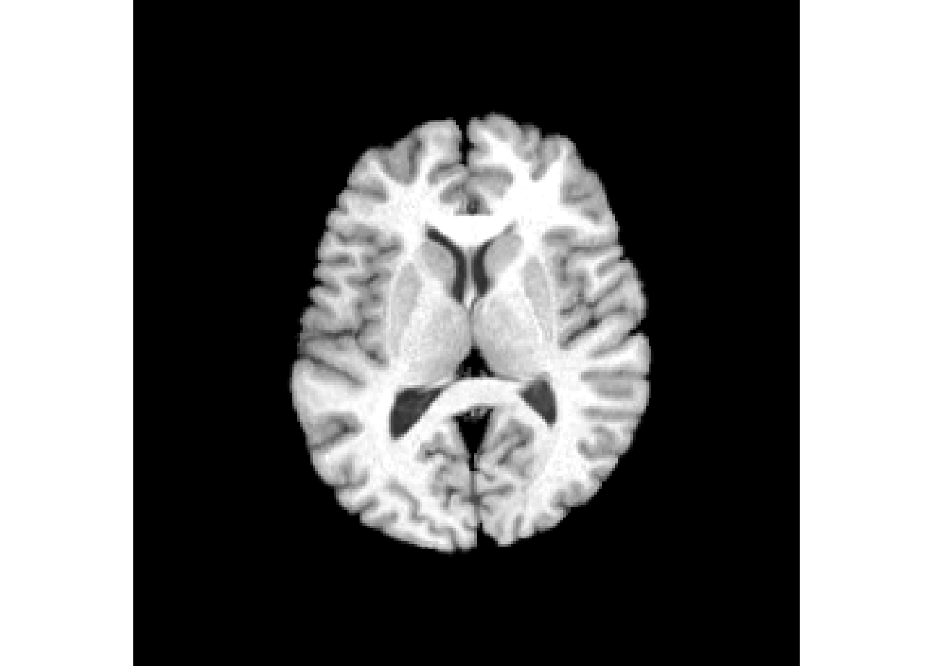
Plot overlay with transparency
antsplot.olay(r16,r64)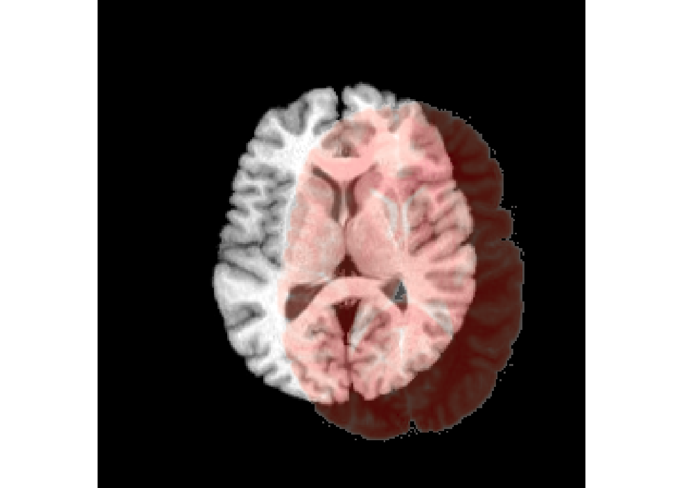
Plot borders of overlay
antsplot.canny(r16,r64)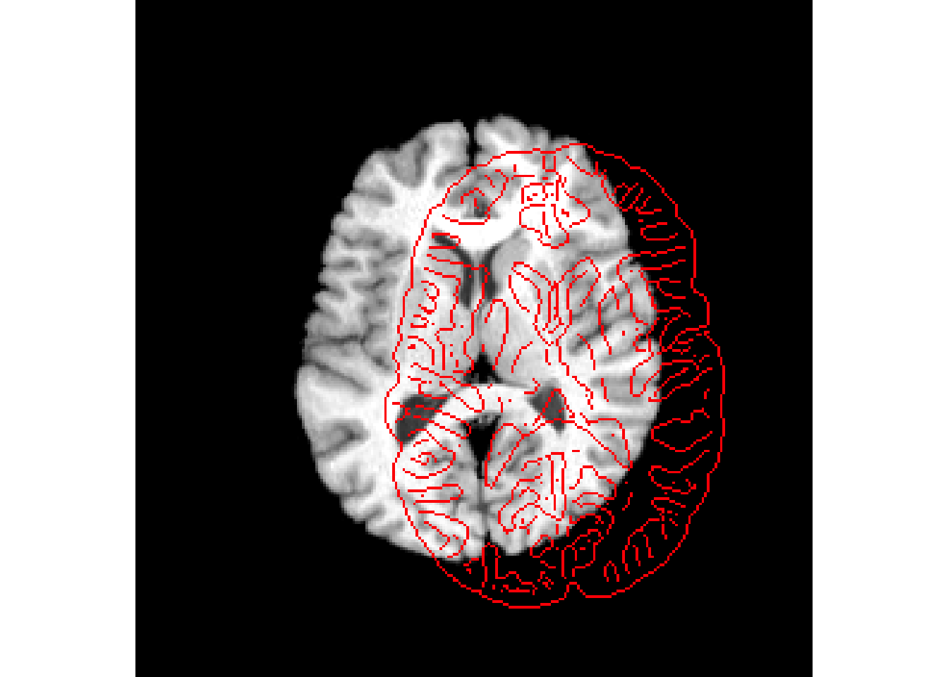
Estimate Registration
See ?antsRegistration() for different typesofTransform
Translation
trans_reg = antsRegistration(
  fixed=r16,
  moving=r64,
  typeofTransform = 'Translation'
)

readAntsrTransform(trans_reg$fwdtransforms)
antsrTransform
Dimensions : 2
Precision : float
Type : AffineTransform antsplot.canny(r16, trans_reg$warpedmovout)
Rigid registration
rigid_reg = antsRegistration(
  fixed=r16,
  moving=r64,
  typeofTransform = 'Rigid'
)


antsplot.canny(r16, rigid_reg$warpedmovout)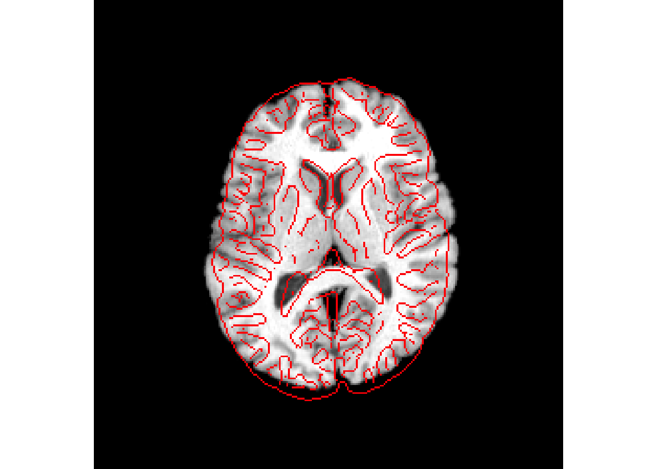
Affine registration
affine_reg = antsRegistration(
  fixed=r16,
  moving=r64,
  typeofTransform = 'Affine',
  verbose = F
)

antsplot.canny(r16, affine_reg$warpedmovout)
SyN registration
syn_reg = antsRegistration(
  fixed = r16,
  moving = r64,
  typeofTransform = 'SyN'
)

antsplot.canny(r16, syn_reg$warpedmovout)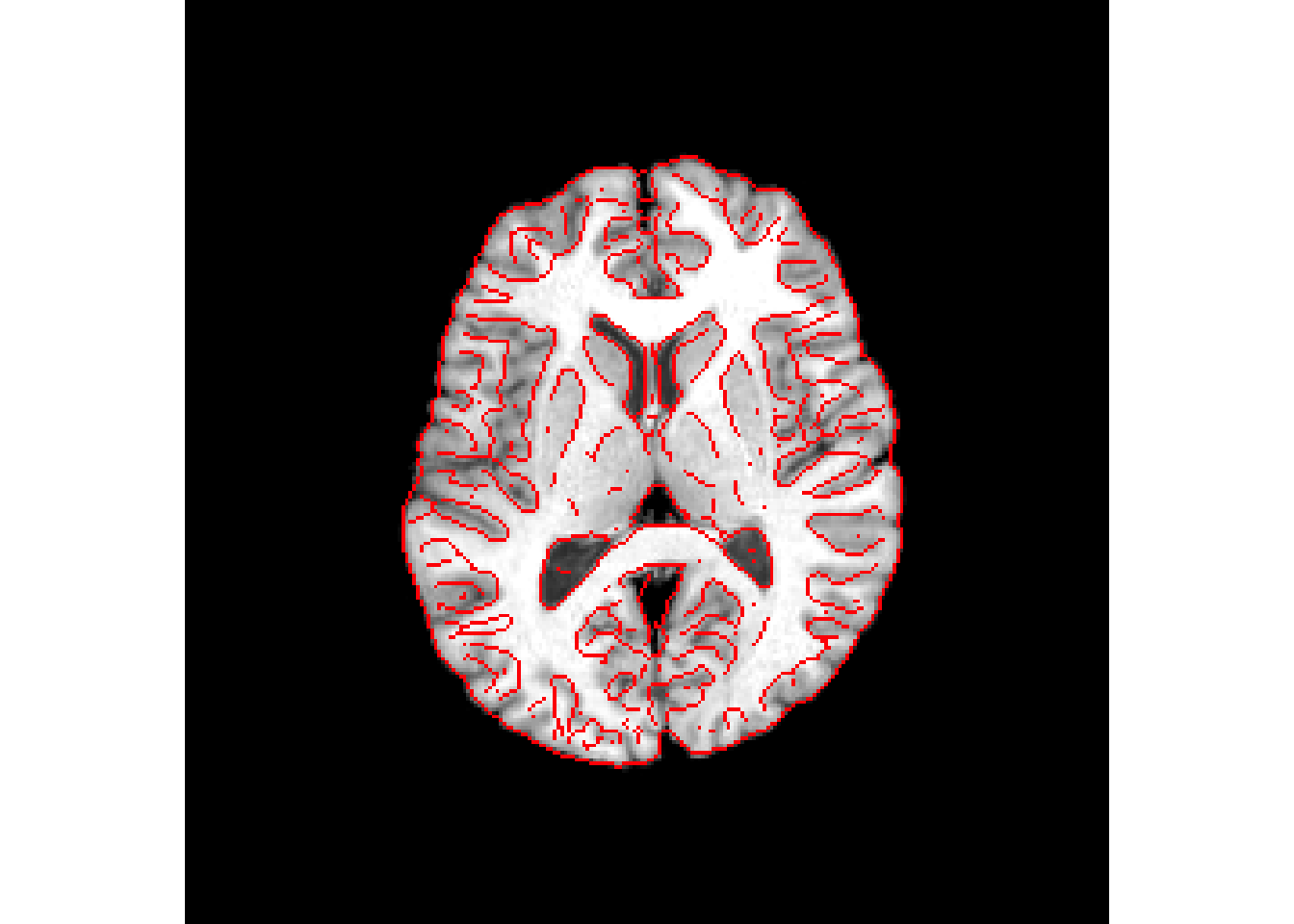
SyNCC registration
synCC_reg = antsRegistration(
  fixed = r16,
  moving = r64,
  typeofTransform = 'SyNCC'
)

antsplot.canny(r16, synCC_reg$warpedmovout)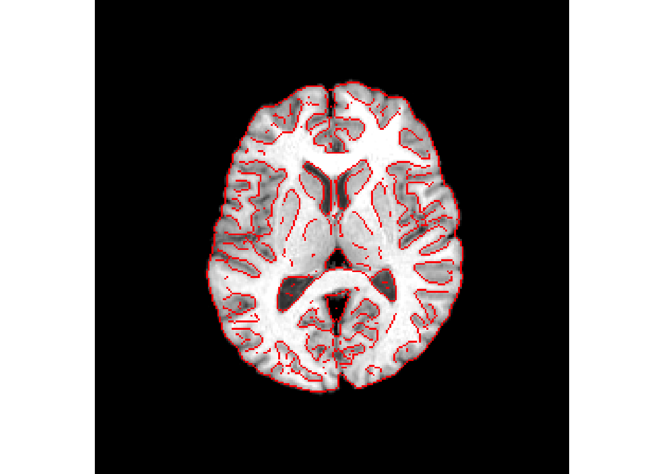
Mutual Information metric
To estimate the goodness of different kinds of registration we can plot the MI metric against the number of parameters
MI <- c(
  antsImageMutualInformation( r16, r64),
  antsImageMutualInformation( r16, trans_reg$warpedmovout),
  antsImageMutualInformation( r16, rigid_reg$warpedmovout),
  antsImageMutualInformation( r16, affine_reg$warpedmovout),
  antsImageMutualInformation( r16, syn_reg$warpedmovout),
  antsImageMutualInformation( r16, synCC_reg$warpedmovout)
)

nparameters = c( 0, 2, 4, 8, 16, 32 )
plot( nparameters, MI, type='l', main='Similarity vs number of parameters' )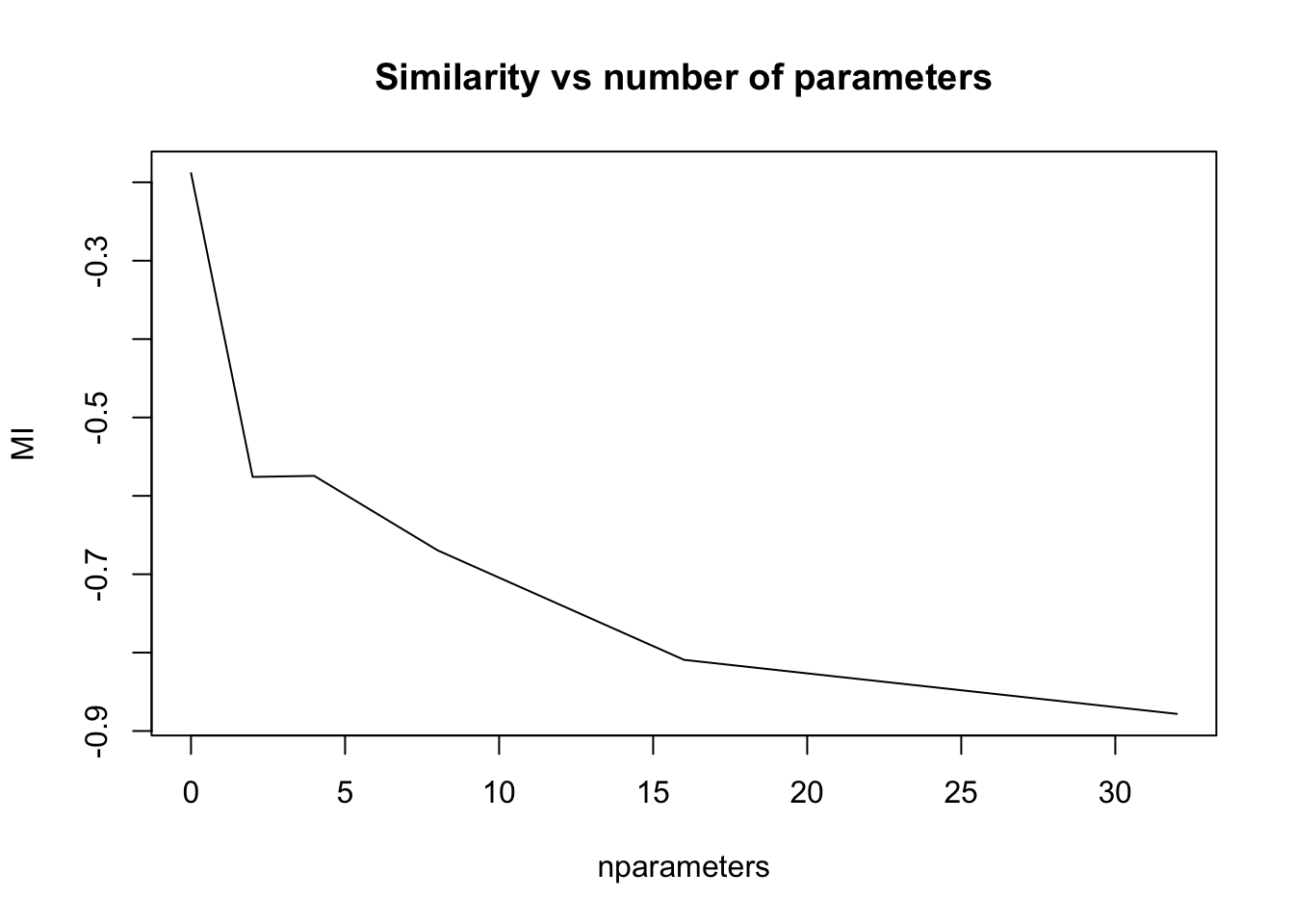
Jacobian determinant image
From Brian Avants’ notebook on antsRegistration:
“What does “differentiable map with differentiable inverse” mean? The diffeomorphism is like a road between the two images - we can go back and forth along it.
It also means that if we compose the mapping from A to B with the mapping from B to A, we get the identity.
We can check this by looking at the result of the composition of SyN’s forward and inverse maps."
Forward warpfield
grid_fw = createWarpedGrid( r16,
                            fixedReferenceImage = r16,
                            transform = syn_reg$fwdtransforms[1]
                          )

invisible(plot( grid_fw ))
Inverse warpfield
grid_backwd = createWarpedGrid( r16,
                                 fixedReferenceImage = r16,
                                 transform = syn_reg$invtransforms[2]
                              )
invisible(plot( grid_backwd ))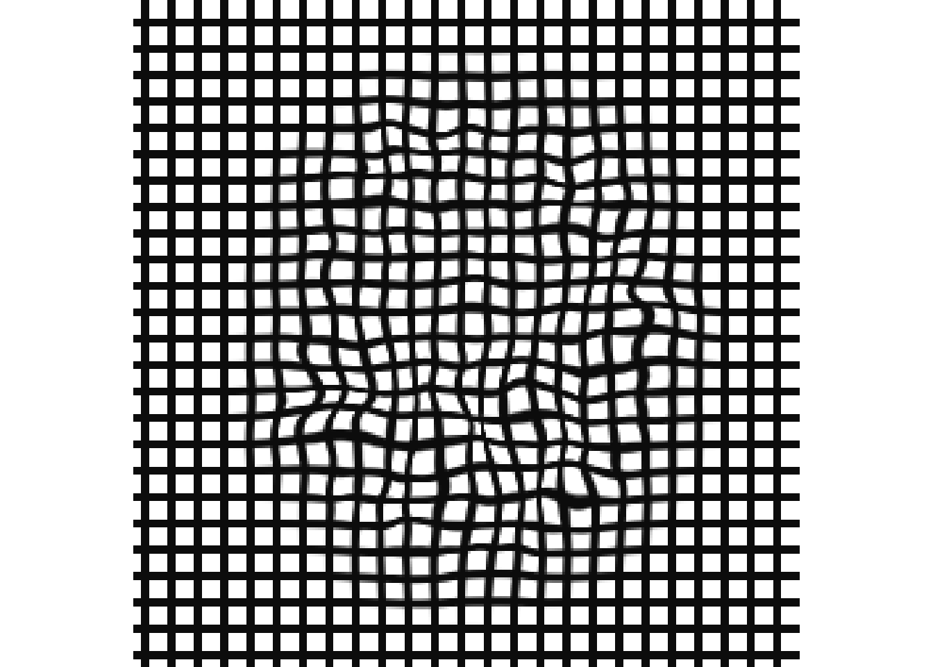
Composition of forward and inverse
emptygrid = createWarpedGrid( r16, fixedReferenceImage = r16 )

invidmap = antsApplyTransforms( r16, emptygrid,
   c( syn_reg$invtransforms, syn_reg$fwdtransforms ),
   whichtoinvert = c( T,F,F,F ))  # tricky stuff here

invisible(plot( invidmap ))
“This “inverse identity” constraint is built into SyN such that we enforce consistency in the digital domain.
What this means is - any “shape change” is encoded losslessly into the deformation field.
Non-diffeomorphic maps may lose information or may be completely uninterpretable, statistically.
One way to check this is to investigate the jacobian. They should be positive which indicates that the topology of the image space is preserved ( no folding and no holes or tears are created )."
syn_reg_jac = createJacobianDeterminantImage( r16,
                                              syn_reg$fwdtransforms[1],
                                              geom = TRUE,
                                              doLog = T)

synCC_reg_jac = createJacobianDeterminantImage( r16,
                                                synCC_reg$fwdtransforms[1],
                                                geom = TRUE,
                                                doLog = T)
Is there a difference between the two jacobians? Paired t-test.
mask = getMask( r16 ) %>% morphology("dilate",3)
print( t.test( syn_reg_jac[ mask == 1 ], synCC_reg_jac[ mask == 1], paired=TRUE  ) )
    Paired t-test

data:  syn_reg_jac[mask == 1] and synCC_reg_jac[mask == 1]
t = 22, df = 19684, p-value <2e-16
alternative hypothesis: true difference in means is not equal to 0
95 percent confidence interval:
 0.050 0.059
sample estimates:
mean of the differences
                  0.054
library( ggplot2 )
n = sum( mask == 1)
# SyN uses MI, SyNCC uses CC
mydf = data.frame(
registration = c( rep( "cc", n ) , rep("mi", n ) ),
jacobian = c( synCC_reg_jac[ mask == 1 ], syn_reg_jac[ mask == 1] ) )
ggplot( mydf, aes(jacobian, fill=registration )) + geom_density(alpha = 0.2)
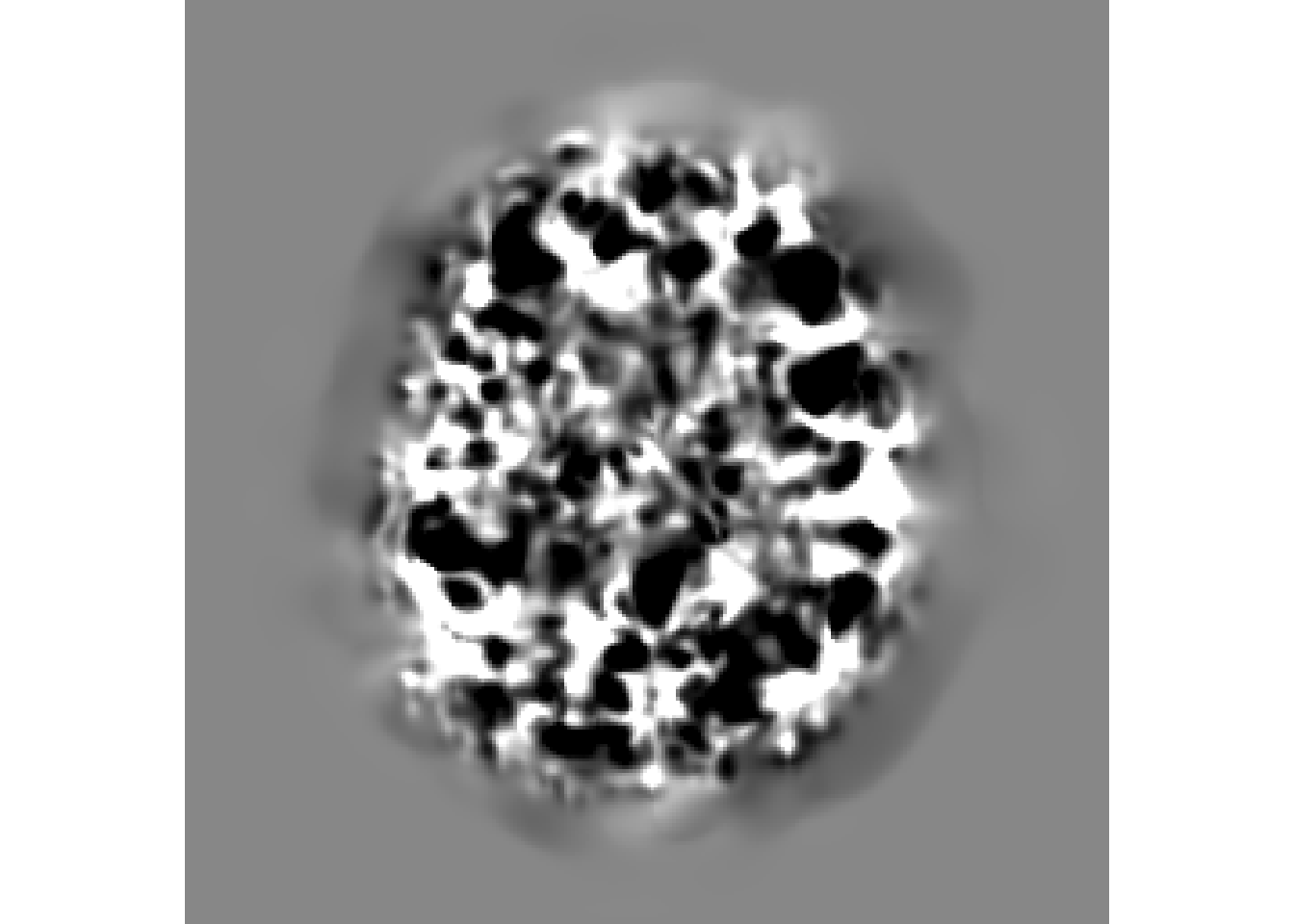
You can also visualize the jacobian determinant image
jac of SyN
antsplot.single(syn_reg_jac)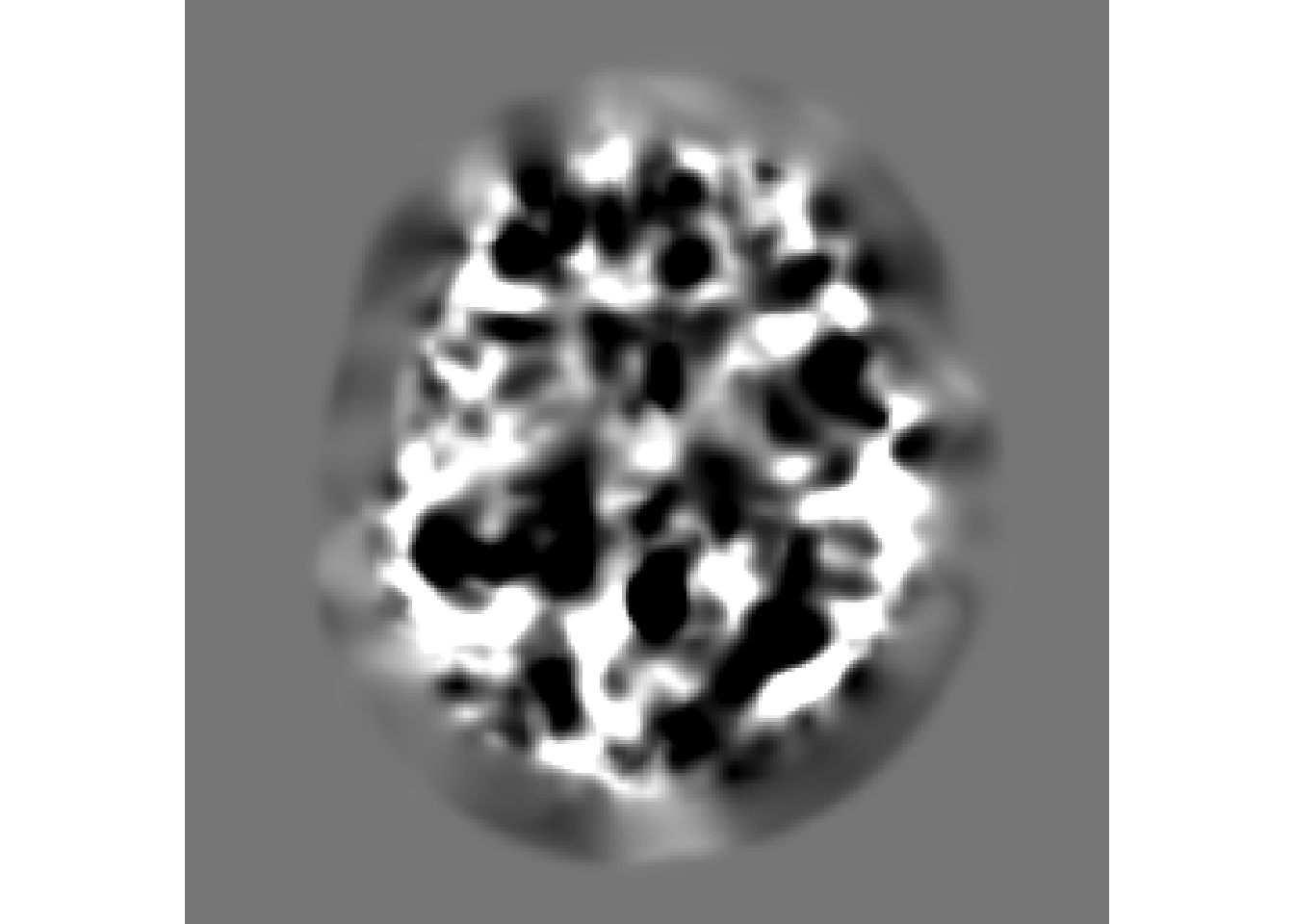
jac of SyNCC
antsplot.single(synCC_reg_jac)