fast NIFTI operations in R
LC
1/17/2021
Intro
I collect here a few notes about carrying out fast operations (well let’s say as fast as possible…) on NIFTI images in R.
A huge inspiration and source of information was the Neuroimaging Analysis with R course by John Muschelli
NB: This is constantly a work in progress, and it will change from time to time.
Load NIFTI image
RNifti is the fastest library I found so far to load NIFTI files
library(RNifti)
library(dplyr)
library(microbenchmark)

# superfast load with RNifti::readNifti
bd <- sprintf("%s/data",getwd())
nii_file <- paste0(bd,"/icbm152_2009_brain.nii.gz")

nii <- RNifti::readNifti(nii_file)
Indexing
hist(nii[nii>0])
Flattening onto a vector
niivec <- c(nii)
Send idx/val of nnz voxels to a data.frame
df <- data.frame(
  idx = which(nii > 0)
  ) %>%
  mutate(val = nii[idx])

df %>% head()
idx val
1 17039 20.91664
2 17040 20.86172
3 17041 20.56490
4 17042 20.86172
5 17043 20.91664
6 17235 21.50880
List of idx and mean val for different ranges of vals
rois <- list(
  roi_1 = 60,
  roi_2 = 71,
  roi_3 = 90
)

lapply(rois, function(x) {
  list(
    roi_numba = x,
    numba_voxels = which(nii > x) %>% length(),
    meanvals = mean(nii[which(nii > x)])
  )
}) %>% jsonlite::toJSON(pretty = T)
{
"roi_1": {
"roi_numba": [60],
"numba_voxels": [1412538],
"meanvals": [73.142]
},
"roi_2": {
"roi_numba": [71],
"numba_voxels": [767138],
"meanvals": [79.658]
},
"roi_3": {
"roi_numba": [90],
"numba_voxels": [353],
"meanvals": [90.4395]
}
}
View slices
With lapply %>% do.call
slices_numba = c(80,90,100)
imlist <- lapply(slices_numba, function(x) nii[ , ,x])
imstack <- do.call(rbind, imlist)
image(imstack)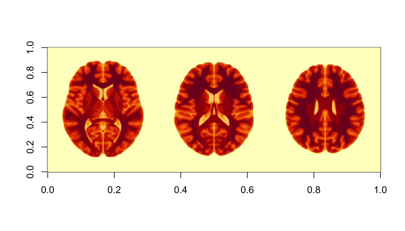
Manual slicing
sl80 <- nii[ , ,80]
sl90 <- nii[ , ,90]
sl100 <- nii[ , ,100]

image(rbind(sl80,sl90,sl100))
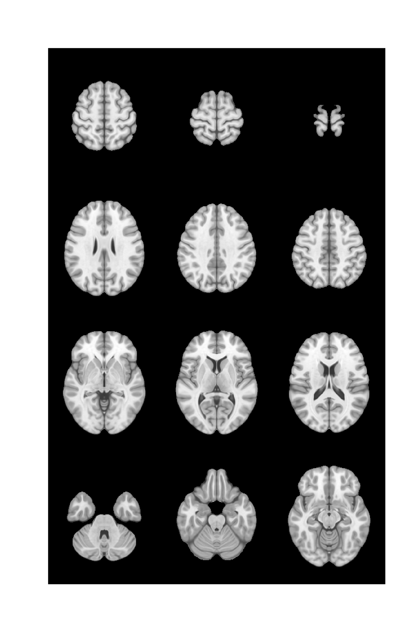
Build a 4x3 montage
library("RColorBrewer")
col <- colorRampPalette(c("black","white"))(256)

slices_numba = seq(40,170,10)[1:12]

imstack <- lapply(slices_numba, function(x) nii[ , ,x]) %>% do.call(rbind, .)

montage <- function(imstack,nr) {
  ist <- imstack
  # length of each row
  xspan <- nrow(ist)/nr

  # dummy to add rows
  sq <- vector()

  # add rows and delete them from ist
  for (i in 1:nr) {
    onerow <- ist[1:xspan, ]  # select one row
    sq <- cbind(sq,onerow)    # add row to sq
    ist <- ist[-c(1:xspan),]  # delete row from ist
  }

  return(sq)
}

montage(imstack,nr=4) %>% image(col=col, axes=F, useRaster = T)